Abstract
This work presents an LLM-augmented engineering process for rapid prototype creation of a high-fidelity Digital Twin for robotic fleet telemetry. We first implement an autonomous fleet simulator comprised of geofence-constrained hazard and path simulators. We then populate a geospatial database, telemetry pipeine, and integrated GIS dashboard for an autonomous thermal-intervention system for the detection and eradication of invasive species. We connect to this isolated service architecture over a private network WebSocket, culminating in a scalable live demo, WeedScorch-Pro, developed for the AgTech divison at Boron Telematics. Finally, we perform an analysis of the user prompts and resulting demo implemention, and create a framework for assessing future autonomous engineering workflows.
Introduction
Designing a Digital Twin often requires extensive system analysis of the target domain alongside the hardware and software engineering constraints associated with this domain. For production-level accuracy, any software-based simulation should simulate the target hardware implementation and the limitations of communication subsystems specified within the boundaries of the system architecture and modeling domain.
Methodology: LLM-augmented Engineering
We created this Digital Twin via a single-threaded, recursive, multi-phase LLM chat session. Certain model outputs were debugged via local LLM, and results from these sessions were used to augment the main LLM chat session. The code was hand-integrated in an iterative manner, with minimal manual intervention. The app was manually deployed to production (with LLM-assisted server configuration). The architecture was built component-by-component with the communication lines fully specified. Leveraging prior knowledge of high-bandwidth communication patterns and geospatial design patterns, certain technology suggestions were injected into the prompts.
Prompting as Role-based Orchestration
We instructed the LLM to derive agentic roles from the prompts specified. The LLM classified the prompts into four distinct categories: Implementation, Tester, Architect, and Reviewer.
| LLM role | Number of Prompts | Engineering Function |
|---|---|---|
| Implementation | 35 | Translating architectural specifications into functional logic |
| Tester | 10 | Generating edge-case scenarios and verifying spatial boundary logic |
| Architect | 6 | Defining system interfaces, schemas, and high-level topology |
| Reviewer | 1 | Final auditing of the integrated service loop |
This classification highlights a high level of instructional density within the Architect prompts. By increasing the depth of these prompts, we were able to reduce the amount of Reviewer cycles to a single prompt. A higher number of Tester prompts relative to the Architect prompts highlights the difficulty of a single-threaded, iterative prompting strategy. Prompts needed to distinguish between high-level constructs and low-level guardrails when designing the Interface Contract.
System Architecture
Note: This drawing is based on a diagram generated by the LLM.
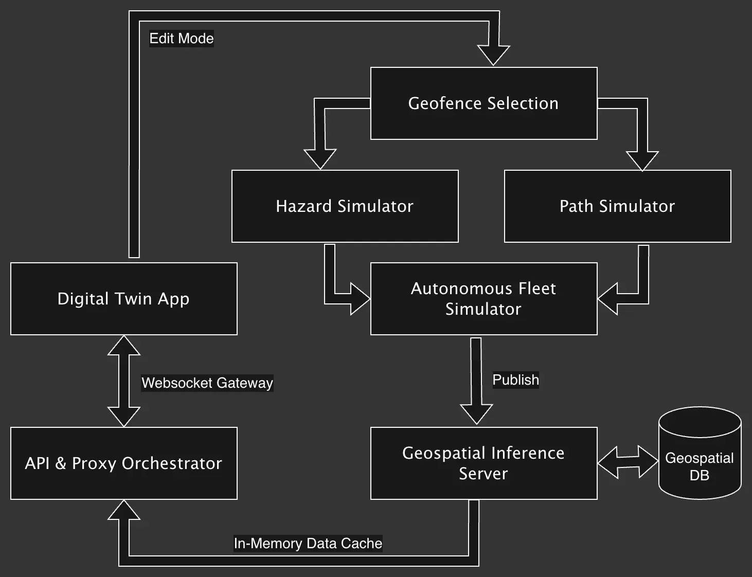
Autonomous Fleet Simulator
The Autonomous Fleet Simulator described here consists of three inputs; the Geofence Selection, Hazard Simulator, and Path Simulator. An Edit Mode is added to the Digital Twin App in order to record coordinates of for the geofence. We record this bounding box in the geofence.json file.
The Hazard Simulator takes this geofence.json as input, reads from a hazard-types.json file denoting the types of hazards to generate (in this case the list of invasive plant species), and then creates a hazards.json as a FeatureCollection of geospatial hazards along the path of the number of bots. This simulates fleet-level detection of hazards.
./hazard-sweep <geofence.json> <number_of_bots>
Likewise, the Path Simulator takes the same arguments, and generates a swath of fleet movement in paths.json, based on the number of bots specified.
./path-sweep <geofence.json> <number_of_bots>
For this simulation, the bot reads its starting position from the Geospatial DB, but then uses paths.json to determine the current fleet trajectory. This technique ensures that when we refresh the page, or open the page in multiple browser windows, the fleet will resume at their last known coordinates. Every copy of the page will then rely on its cached trajectories for hazard clearance. In an environment where real-time fleet positioning is available, we can cache path information from the geospatial database in a similar way, allowing us to generate offline playback files for analysis that do not require server access.
API & Proxy Orchestrator
We coordinate a WebSocket connection between with the Digital Twin App and the Geospatial Inference Server via the API & Proxy Orchestrator. This abstraction allows the backend telemetry server to communicate internally on the backend network with the isolated geospatial database without exposing either to the public demo interface.
Implementation Analysis & Trade-offs
The prompt analysis was conducted post-implementation, once the demo was finished. The analysis itself was assisted by a local LLM with access to the demo source code, and a ~9000-line session history that lacked any annotations as to input or output. From an original assessment of 14 domains, we instructed the model to derive and restrict the prompts to six core functional domains; Simulation Engine, Reliability & Debugging, Geospatial Infrastructure, Interface & Presentation, State & Persistence, and Telemetry & Monitoring. Charts were developed by an LLM-generated program based on the extracted data.
Prompt-to-Implementation Distribution by Functional Domain
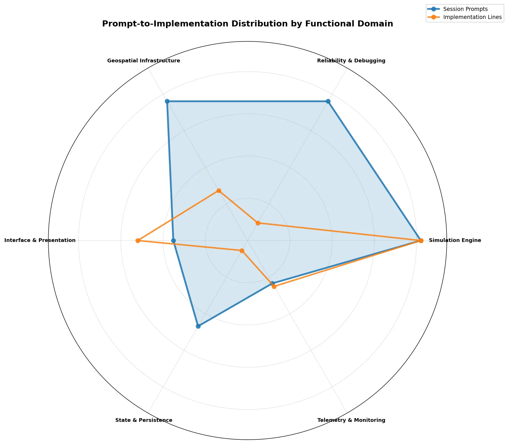
From the chart, we see a clear decoupling between Prompt (representing the human instructional input), and Implementation (representing the model output). The high prompt-to-implementation ratio for the Simulation Engine shows that the model frequently required elaborate prompting to create a successful implementation. This also hints, as we will see in the next graph, that this was the area of highest intensity effort. In contrast, we see the implementation lines drop far below the prompting area for the Geospatial Infrastructure and Reliability & Debugging domains. This behavior may represent heavy architectural refinement where more effort was expended for fewer results. The Telemetry & Monitoring mirrors the prompt-to-implementation ratio of the Simulation Engine, but at a more peripheral touch point. Likewise, the State & Persistence domains also suggests a lower touch point, but with more refinement needed. Finally, we see the implementation line exceed the prompt space for the Interface & Presentation domain, indicating that the model was highly-efficient at generating boilerplate UI from generic prompts without micro-managing UX decisions.
Distribution of Development Metrics by Domain
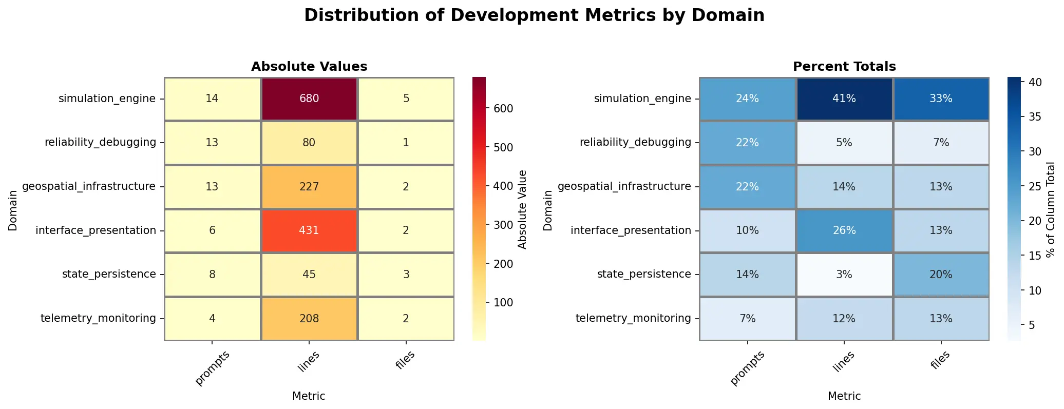
Here the heatmap clearly shows the hot spots of activity (Simulation Engine, Interface & Presentation, Geospatial Infrastructure). We can drill down further into the data by developing metrics to determine the efficiency of the work. These metrics can then be used to plan further agentic tuning to better formulate Ralph loops for autonomous coding.
Development Metrics
Note: These metrics were derived by a local LLM based on the heatmap.
| Domain | Efficiency | Friction | Density | Reach | Status |
|---|---|---|---|---|---|
| Simulation Engine | 48.6 | 2.8 | 136 | 0.36 | Core Development |
| Reliability/Debug | 6.2 | 13.0 | 80 | 0.08 | High Friction/Bottleneck |
| Geospatial Infra | 17.5 | 6.5 | 114 | 0.15 | High Output |
| Interface/Pres. | 71.8 | 3.0 | 216 | 0.33 | High Velocity/Automated |
| State/Persistence | 5.6 | 2.7 | 15 | 0.38 | Low Touch |
| Telemetry | 52.0 | 2.0 | 104 | 0.50 | Peripheral |
Prompting Efficiency (Lines per Prompts)
The ratio of the number of lines of code generated to the number of prompts. This can be seen as the effective yield. How efficient is the amount of human effort and token budget that we are spending to complete the task? How complex is the work?
Debugging Friction (Prompts per File)
This ratio of the number of prompts to the number of files generated. How difficult is the development process? How much human intervention is needed?
Structural Density (Lines per File)
The ratio of the number of lines of code generated to the number of files generated. This is a measure of how granular (or bloated) the implementation is. What is the size of the logic chunks being generated? Are we creating a monolithic architecture comprised of large, single-purpose files? Are we decoupling boilerplate-heavy code into modules?
Instructional Reach (Files per Prompt)
The ratio of the number of files to the number of prompts. How much impact are the prompts having? Are we micro-managing the model or providing high-level architectural guidance?
Conclusion
Designing a functional Digital Twin via LLM-augmented engineering is a challenging exercise, not only is domain knowledge needed, but also software engineering knowledge, or at the very least, knowledge of the model's capabilities and capacity. The app presented here was developed in a naive way, and still produced functional results. The metrics developed for the implementation analysis are valuable beyond this project, and can be used to evaluate both new projects and future iterations of this project. Classification of the prompts into agentic roles further solidifies the approach, and can be used to bootstrap additional workflows.
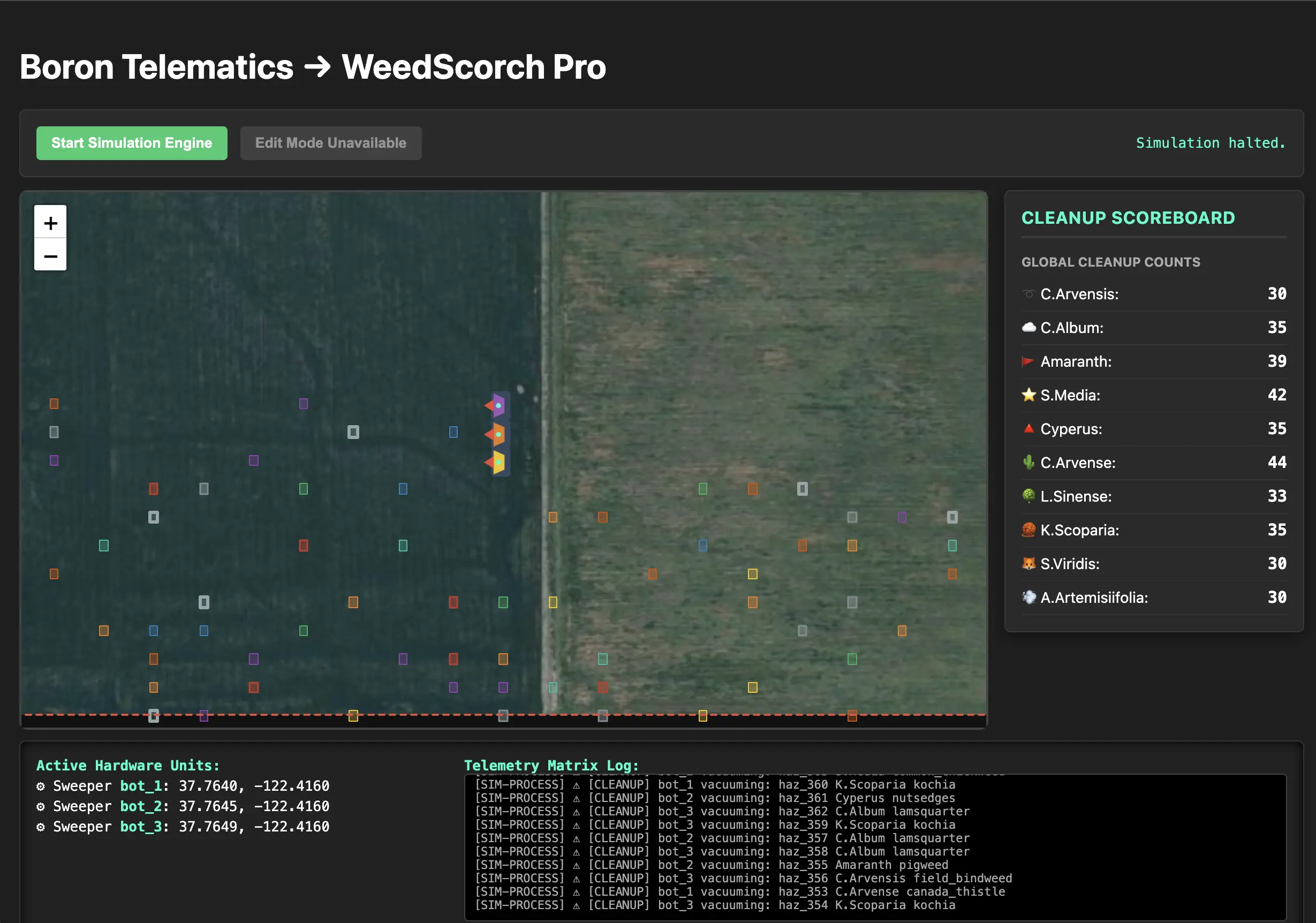
The Digital Twin App is live at WeedScorch-Pro.
Limitations
To ensure deterministic performance for the demo, the Edit Mode is currently turned off on the live site. This creates a static geofence for a consistent experience against all open browser sessions. The Autonomous Fleet Simulator also makes several assumptions concerning the Hazard and Path simulators. Although they are first-class geopsatial objects, Hazards are not currently not persisted to the database, and this was done to allow full browser refresh of hazards on demand. When the robots reach the end of the geofence, they will retrace the path backwards (right-to-left, bottom-to-top) back to the beginning, even after all the hazards have been cleared. Additionally, while a browser refresh will then reset the hazards, it also resets the fleet to proceed in the original top-to-bottom, left-to-right direction.
Acknowledgements
The geospatial challenges and system constraints addressed in this prototype are derived from the operational domains of autonomous weed identification and mitigation, as exemplified by the architectures of AgTech platforms such as Carbon Robotics, Naïo Technologies, and Farmwise. The top ten list of invasive species for this demo was compiled from GVC Farm Supply.